0:00Hey, it's Tim here and in today's video we
0:03're taking on one of the most requested
0:03videos
0:04on this channel and that is the topic of
0:06level of detail calculations. Today we're
0:08starting with
0:08the fixed level of detail calculation and
0:11before we get stuck into the video just a
0:12quick reminder
0:13that if you like the videos that I share on
0:15my channel please do share them with other
0:16people,
0:17like, subscribe and hit the notification
0:19bell so you can get the notifications when
0:21I upload
0:22new videos. Okay without further ado let's
0:24get stuck in. Okay so over the last couple
0:26of days
0:26I've actually uploaded two videos on my
0:28channel that cover some concepts that we're
0:30going to use
0:31today so if you haven't had a chance to
0:32check those out these are the two videos
0:34that I'm
0:34referring to. The first one is an
0:36introduction to order of operations. This
0:38is important because
0:39we're actually going to be using that
0:40technique to understand which level of
0:42detail calculation
0:44we should be using. The other video is
0:46about understanding the granularity in your
0:48data set,
0:49essentially understanding what does each
0:51row represent in your data set. That's also
0:53another
0:53key concept to understand really really
0:55clearly before you start working with LODs.
0:57So if you
0:58haven't had a chance to check out those
0:59videos or even just understand those topics
1:02in general,
1:02go out to YouTube, go out to Google and
1:04understand those topics in detail because
1:06you'll need those
1:07concepts in this video. Okay let's head
1:09back to Tableau and let's open up a very
1:12simple
1:12visualization. We're actually going to
1:14build one ourselves. We're just going to go
1:15into Superstore
1:16here and we're going to select the American
1:18version which is the second one. If you don
1:20't
1:21see that one just connect to whichever
1:22version that you have available and you
1:24should get
1:24something like this. Now when we work with
1:26visualizations in Tableau there's this
1:29concept
1:29called the viz level of detail and the viz
1:32level of detail is essentially the level of
1:34detail that
1:35we have in our visualization. Now there's
1:37something I'm really conscious of in this
1:38video which is how
1:39many times can I say level of detail before
1:42actually explaining level of detail and so
1:44I
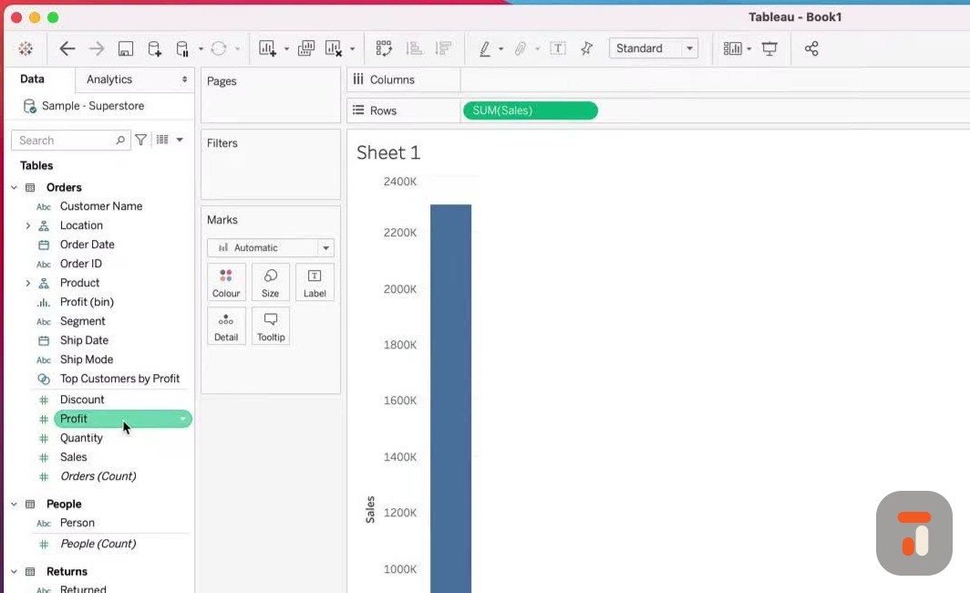
1:44want to do that right now. Okay so in our
1:47visualization let's just build a very
1:48simple
1:49chart. Let's bring sales onto rows and then
1:52let's bring a subcategory onto columns.
1:55Okay so we've got a very simple
1:57visualization here and in essence the viz
2:00level of detail refers to
2:02certain dimensions that we have in certain
2:04places in our visualization. Let me try and
2:07highlight
2:07that for you. If I just grab my highlighter
2:09here and I just highlight the squares that
2:11represent
2:12sort of the viz level of detail that you
2:14should be aware of and the first is of
2:15course the columns
2:16and rows. Any dimensions that you put into
2:18these two groups will fundamentally change
2:20the level of
2:21detail that we have in our visualization.
2:23What do I mean by that? Well let me show
2:24you if I then
2:25drag category onto columns you'll see that
2:28my visualization changes to add the
2:31category here
2:32into the level of detail that I'm seeing in
2:34my visualization. There is however more
2:36detail and
2:37granularity in this data set it actually
2:39goes down to the product level but if I put
2:41anything here on
2:42the columns and rows you'll see that it
2:44changes my visualization. Okay now you can
2:47change your level
2:48of detail very easily just by putting
2:50dimensions in other places. So for example
2:52if I was to drag
2:53a subcategory here and put it onto color
2:55you'll see that that affects my
2:57visualization and if I
2:58was to then remove it from the rows you'll
3:01see that it still remains in my chart but
3:04this time
3:05as represented by color. So the subcategory
3:08although it's not in the chart is still
3:10controlling the viz level of detail that I
3:12've got here essentially working at the
3:14category and the
3:15subcategory level. If I was then to hit
3:18plus again you'll see that this now goes to
3:20each and every
3:21manufacturer so you can see that this is
3:23actually split out. If I change the colors
3:25here a little
3:25bit you'll see that actually we can see a
3:27lot more manufacturers and so although my
3:29chart hasn't
3:30changed it's still the same bar chart it's
3:32still the same totals the level of detail
3:35is changing
3:36each and every time I add a new dimension
3:38onto the color or the detail pane you'll
3:41see that these two
3:42are actually on the detail pane as shown
3:44essentially by this mark you can just see
3:46that this
3:47icon here is exactly the same as these two
3:49okay so just something to be aware of
3:51anytime you add
3:52something to the marks pane and the columns
3:55and rows it changes. The only exception in
3:57fact is
3:58actually this one here the tool tip so if I
4:01was to just essentially put something onto
4:03the tool tip
4:04let's say I put segment onto tool tip you
4:06'll see this doesn't change my level of
4:08detail in my
4:09visualization so let's just drag these two
4:12away so you see we've just got subcategory
4:14and then here
4:15we've got segment here in the in the tool
4:17tip and you'll see that it hasn't changed
4:19anything and if
4:20I hover over you'll actually see that it
4:22uses a star and this is actually in
4:24relation to something
4:26else called the attribute function of
4:27course you've guessed it I've already made
4:29a video about
4:30this on my channel so go check that out if
4:32you want to know more about why it uses a
4:34star and
4:34not actually list out the segments okay so
4:37we now understand what changes the visible
4:39level of detail
4:40if I just go here to a line there is
4:42another one that can sometimes happen so it
4:44's essentially
4:45these these ones in the top row here the
4:48label the detail and essentially the path
4:51and then anything
4:53obviously we've got in our visualization
4:55and then lastly the columns and rows okay
4:57so these are the
4:58places that can change the level of detail
5:01in our visualization everywhere else doesn
5:04't change the
5:05visible level of detail is essentially
5:07happening elsewhere it doesn't change what
5:08we see visually
5:09so that's the first thing to understand
5:11what is the visualization's level of detail
5:14okay now this is
5:15important because when we start asking
5:17questions of our data we need to be able to
5:19understand what's
5:19actually going on so let me go to a new
5:21sheet and just pose a sort of a new
5:23challenge to you
5:24and this is actually going to be a good use
5:26case for the fixed level of detail that we
5:27'll come to
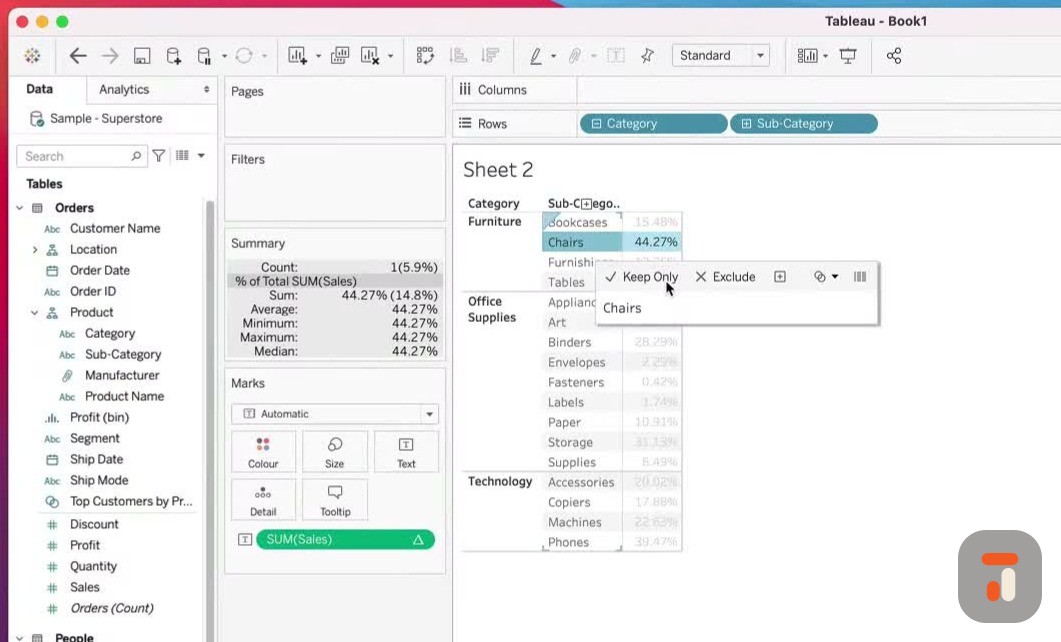
5:28very soon so let's just drag subcategory
5:30onto rose I'm going to drag category and
5:33put it in front of
5:33it and then I'm going to drag sales and
5:35this time I'm just going to put it on this
5:37table here okay
5:38last thing I'm going to do is go to works
5:40heet and show the summary window and then I
5:42'm just going to
5:42drag the summary window here to the left
5:44hand side underneath my filters pane so it
5:46's nice and easy
5:47to see now the interesting thing here is if
5:49we wanted to calculate the percentage of
5:52total within
5:53each category for each subcategory then I'd
5:55essentially need to understand the context
5:58of
5:58what the total was so if I go here and just
6:00select category you'll see that the total
6:03here is 742
6:04000 if I just expand this over here you see
6:07the summary window is like a calculator if
6:09we click
6:09on something it does a bunch of aggreg
6:11ations for us and just gives us the value if
6:13I go to office
6:13supplies it's 719 000 if I go to technology
6:17it's 836 000 okay and so what I can very
6:20easily do in
6:21tableau is just go in here create a quick
6:23table calculation and select percentage of
6:26total now
6:27what will actually happen is it will do a
6:29percentage of total across the whole data
6:31set
6:31essentially okay and in this case we don't
6:33actually want that we just want one for
6:35each
6:35category so in this one I'm going to cheat
6:37a little bit and I'm going to say compute
6:39using the
6:40pane and I'm just going to leave it at that
6:42okay now the pane in tableau is essentially
6:46this
6:46particular window here if I just highlight
6:48that there you can see it very very clearly
6:50and so what's important here is that this
6:51percentage is essentially going to add up
6:53to 100
6:54when I'm looking at the category so let's
6:56just do that if I click on category you'll
6:59see here that
7:00the sum is 100 for the percentage of total
7:02sum of cells and for the whole table it
7:05sees 300
7:06because essentially there's three panes
7:08here in the visualization which adds up to
7:10300 okay now
7:12the frustrating thing is let's say I want
7:14to keep these percentages of totals whilst
7:16only looking at
7:17certain subcategories let's say I always
7:19want to know the percentage of total for
7:21the category
7:22within the subcategory when I only look at
7:24chairs now if I was to exclude everything
7:26and just keep
7:27just chairs you'll see this percentage
7:30changes to 100 and fundamentally this is
7:33caused by two
7:34problems the first one is to do with order
7:37of operation now the order of operations
7:39dictates
7:40that essentially filters and certain
7:43calculations happen in a specific order
7:46check out my other
7:46video on this topic to find out more but
7:49essentially what we're doing when we add
7:51that chair filter
7:52is we're essentially doing this we're
7:54running a dimension filter and the problem
7:56we have is that
7:57our totals and all our aggregations are
7:59actually calculated much further down here
8:01so if you just
8:01go in here we're looking at quick table
8:03calculations actually operating at this
8:05level of information
8:06down here and so the difficult challenge is
8:09how do we keep the context of the question
8:12we're asking
8:14whilst also using a filter which is
8:15actually happening before the calculation
8:18that I do
8:18well this is where level of detail
8:20calculations are really handy because they
8:23they actually have
8:23a different position in the terms of the
8:25order of operations in terms of when they
8:27run so if I
8:28just change to red here and I just
8:29highlight a few things you can see that the
8:31fixed level of detail
8:33actually runs before any dimensional
8:35filters that we might have in our data set
8:38you can see right
8:39here it just runs in between context
8:41filters and dimensional filters okay so we
8:43're actually going
8:44to take advantage of this little quirk and
8:47we're going to use it to solve the answer
8:49that we're
8:49trying to find out which is what is the
8:51percentage of total for a particular sub
8:53category of the
8:55category when we're only looking at one sub
8:57category okay let's switch back to tableau
9:00and have a look
9:00at that question let's just clear the
9:02annotations off the screen here okay so I'm
9:04just going to keep
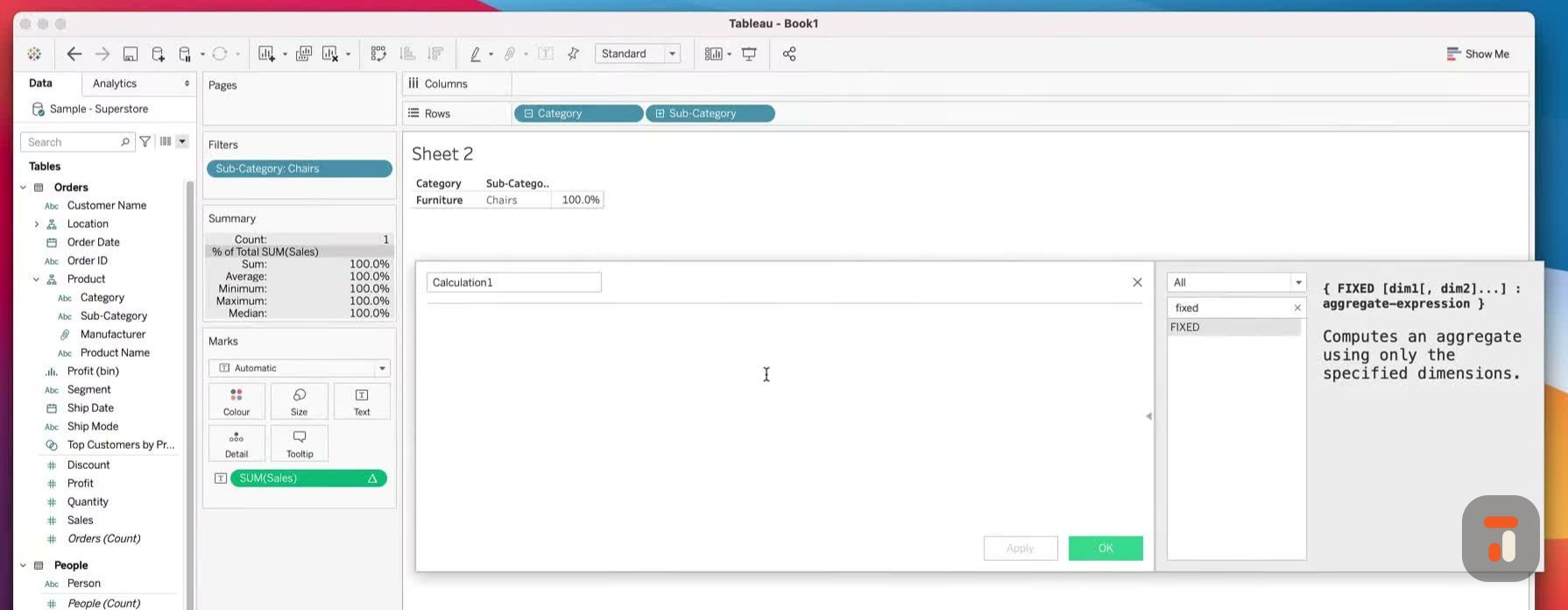
9:05chairs into the visualization and what we
9:07're going to do is we're going to open up a
9:08new calculated
9:10field and if you've never looked at LODs
9:12before that's fine in all my function
9:14videos I've actually
9:14been highlighting the fact that you can
9:16look at any function and see how it should
9:18be written and
9:19how it's used just by opening up this
9:21little side pin here on the right hand side
9:23and essentially
9:24going to that function and seeing how it
9:26should be used in this case we're using
9:28fixed so let me
9:29type in fixed and select that right there
9:31you'll see that actually here on the right
9:33hand side
9:35it has a very sort of strange notation it's
9:36one of the functions that actually uses a
9:38curly brackets
9:39to start it off and then you have to
9:41declare your dimensions that you want to
9:44basically target in
9:45terms of your level of detail and then the
9:47aggregation and then you close it off
9:49essentially
9:49so let's have a go at writing a calculation
9:51I'm just going to write it first then I'll
9:53explain it
9:54after I've written it okay so let's just
9:56first make this larger so you can see it
9:58very clearly
9:59and I'll just go in here and I'll type
10:01curly brackets to open the level of detail
10:04I'll then type fixed and then what we're
10:06essentially asking Tableau to do is to
10:09control
10:09the level of detail based on the dimension
10:12I'm about to declare now okay so in this
10:14case I'd
10:14like to do this for the entire category I
10:17basically want to know what the category
10:20total is so that I
10:22can use that in my calculation okay so
10:25fixing the level of detail of category I
10:27want you to go and
10:28calculate the sum of cells and this is
10:30actually no different to what we would have
10:32normally done
10:33let's just do that there close off the
10:35curly brackets and then do one more just to
10:38close off
10:39the entire LOD okay so you can see here
10:41that this LOD is actually valid you can see
10:43that right here
10:44at the bottom and so now the key thing here
10:47is that essentially we need to sort of just
10:50walk
10:50through this and understand what is going
10:52on okay so let's do that the first thing I
10:54want to do is
10:55just sort of highlight the notation for an
10:57LOD okay the first thing you have are these
10:59curly
11:00brackets at the beginning at the end these
11:02essentially open and close an LOD
11:03calculation
11:04okay now depending on the LOD that you
11:06write the next bit is actually about
11:09telling Tableau what
11:10kind of level of detail you'd like to run
11:13in this green section here you'll see that
11:15it says fixed
11:16at the moment but you can actually have two
11:18other types in this video I'm only looking
11:20at fixed the
11:21other two types are include and exclude
11:24okay now the next thing that comes after
11:26that is actually
11:27this which is essentially us declaring the
11:30level of detail and in the context of fixed
11:33it's nearly
11:34always something that can either be in the
11:36visualization or can be outside of the
11:38visualization
11:39level of detail and the unique thing about
11:42the fixed level of detail is that it acts
11:44independent
11:45of what's happening in the visualization
11:47unlike include and exclude which take what
11:49's in the
11:50visualization into account fixed is the
11:52only level of detail calculation that acts
11:54independent
11:56of what's in the visualization even if it's
11:59at the same level of detail as the
12:01visualization if that
12:02makes sense so you'll see here we do
12:04actually have category in the visualization
12:06but this calculation
12:07is independent of that category if we were
12:10to take it out it would still behave
12:12correctly okay the
12:14next thing we need to do is essentially our
12:16aggregation and that's what we have here
12:18some
12:18of cells and this is actually just what we
12:20do normally it's the same way we'd write
12:21any
12:22calculation okay so we have these
12:24constituent parts of an lod calculation and
12:27essentially
12:27they help us tell tableau how we'd like the
12:30aggregation done and at what level of
12:32detail
12:32we'd like it done at okay and so as i've
12:34said with the fixed one essentially we're
12:37controlling
12:37this at the category level this is going to
12:39happen independent of the visualization and
12:42lastly it's
12:42going to happen it's going to happen before
12:45this filter here which is a dimension
12:47filter so it's
12:48going to happen before this filter is done
12:50which means it will keep the context of the
12:52total and
12:53have the correct number so let's go ahead
12:55and hit apply in fact let me just type in
12:58fixed lod here
12:59and let's just hit apply and click ok and
13:02now when we drag the fix lod into the view
13:06you'll see
13:07something new okay remember the number that
13:10we saw earlier on it was 742 000 now just
13:13to clarify that
13:14let me go ahead and remove this subcategory
13:16filter for chairs and if i click on
13:19furniture you'll see
13:20that this sum now says 2.9 million well
13:22that's because it's adding everything in
13:24here and it's
13:25sort of kind of going crazy so let's just
13:27clear the um let's just clear the table
13:29calculation that
13:30was in there and let's just select these
13:33values here so one two three and four and
13:35you can see
13:36it's 742 000 and that's the exact same
13:40value that we've got here okay so now when
13:43i just keep chairs
13:44in my view notice how tableau remembers the
13:46value because essentially it computed that
13:49number before
13:50it filtered it out of the data set and so
13:52that's the really important thing here it's
13:54doing that
13:55calculation and then it's keeping that
13:57level of detail in context essentially as
13:59we do other
14:00computations so this makes it very easy to
14:03always start telling a story about your
14:05data set at
14:06different levels and also sort of relating
14:08your numbers to different sets of context
14:11okay um now
14:12let's go ahead and finish this calculation
14:14to actually find out what the percentage of
14:16total
14:16should be before um you saw this actually
14:19change to 100 so if we go back here to a
14:22percentage of
14:23total you can see that it's operating at
14:25100 which is of course incorrect we
14:27actually specifically
14:28had it using the pane so let's just keep
14:30that the pain so we can see that it's
14:32working correctly
14:33and now let's finish our calculation in
14:35order to do this i'm going to create a new
14:38calculation
14:39field and in here i'm actually going to
14:40bring in the two things that i've used
14:42before so the first
14:43thing i'm just going to do is sum of cells
14:46and i'm just going to type in cells here
14:48and i didn't
14:49do that correctly there you go so there we
14:51have some of cells and if we expand this
14:53what we're
14:54going to do is we're going to divide the
14:56sum of cells in the view level of detail
14:58against the
14:59calculated fixed level of detail for the
15:01category okay so this is interesting
15:03because i'm not
15:04actually specifying the level of detail for
15:07one of my calculations but in this other
15:09one
15:09i am actually going to be using the fixed l
15:12od which will give us the value for the
15:15category so
15:16this one is actually not listening to the
15:18visualization it's just going to be looking
15:21at
15:21category and i know that here because if i
15:23just click in it and i highlight this to
15:25you you can
15:26see that this is my fixed lod working in
15:28the background okay so this is going to
15:31allow us to
15:32do a couple of things it means is as my
15:34visualization changes the context and the
15:36percentage of total will always be computed
15:38against the category which is really really
15:41important because if i start doing crazy
15:43things with my visualization i know this
15:45number is going
15:45to be correct okay so let's just say that
15:49this is going to be um viz lod sum of cells
15:54divided by
15:56the category sum of cells okay which will
16:00give us a percentage of total against the
16:03category okay
16:04so let's just hit apply and now you'll see
16:06that this new calculation is just shot all
16:09the way
16:09over here and it's now ready for usage okay
16:12so let's go ahead and click okay and let's
16:15bring
16:15this into my view so i'm just going to drop
16:17that in there and you'll see that it says
16:19zero and
16:19you're probably thinking ah what's happened
16:22here why is this failed well let's think
16:23about what we
16:24just did if we edit this calculation we
16:26essentially created a percentage and
16:29because the number is so
16:30small it's essentially rounding it down to
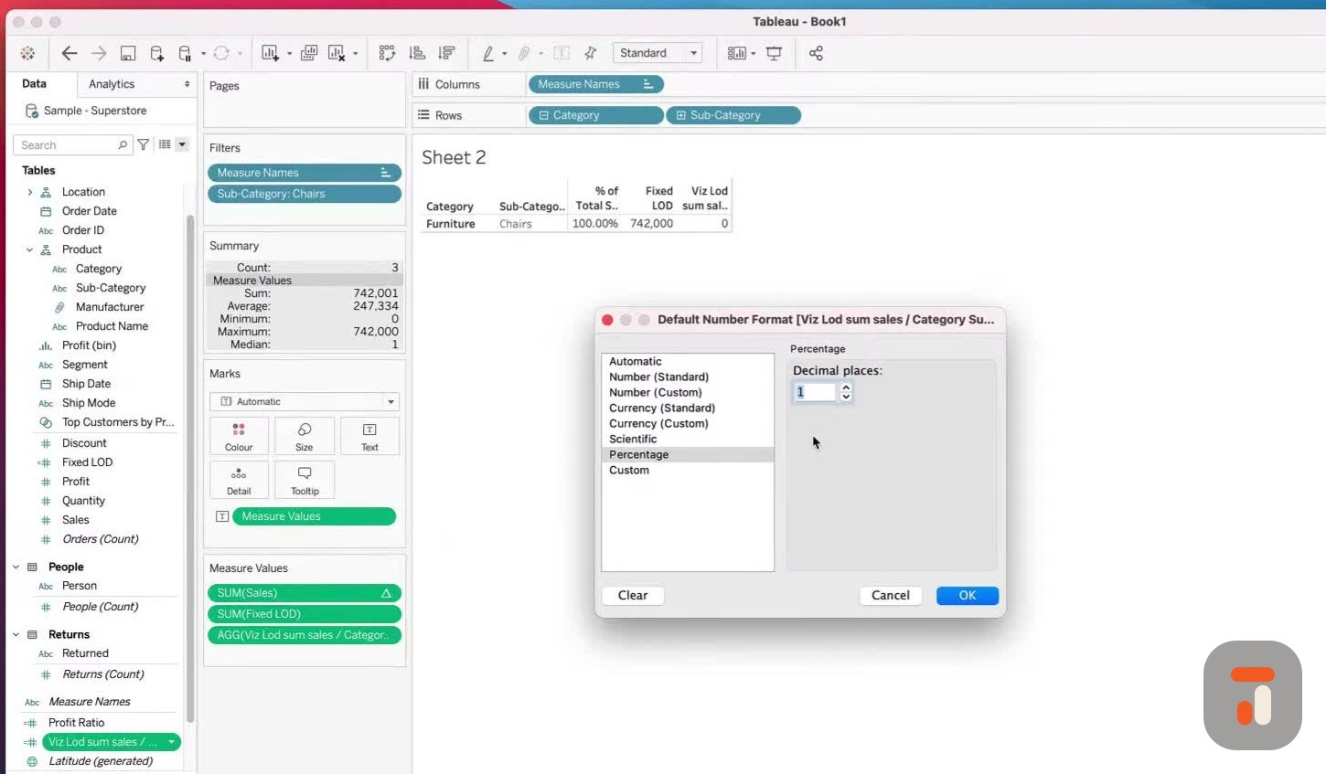
16:33zero so what we need to do is to change
16:35this to a
16:36percentage let's go to default properties
16:39here number format then percentages and we
16:41're just
16:42going to put it at one decimal place here
16:45click okay and now you'll see it says 44.3
16:48percent okay
16:50now this is the moment of truth i'm going
16:52to remove the chairs from the filters pane
16:55we're
16:55going to see if this 44 matches with what
16:57used to say 44 here but now this is 100
17:01because it has no
17:02context of the category so let's go ahead
17:04and remove that and there we have it you
17:06get an exact
17:07same number so it says 44.3 because
17:10fundamentally i've set my number of decimal
17:12places here to one
17:14if i set it to two you'll see it's exactly
17:17the same number 44.27 44.27 so now you can
17:21start to
17:21see the power of an lod specifically the
17:24fixed lod because in this context it's
17:27essentially
17:27allowing us to take a calculation that
17:29actually is in the view we have category
17:31here in the view
17:32but because of the way the calculation
17:34works it's allowing us to move it up in the
17:36order of
17:37operation actually keep the correct value
17:39and then have that in context for another
17:41calculation that
17:41we're going to be using okay now in this
17:44example that's sort of just one quirk i'm
17:46basically using
17:47to get around the order of operations but
17:49in other contexts you might actually use it
17:52to answer
17:52slightly different questions and so that's
17:54now what i'm going to do i'm going to show
17:56you a
17:56couple of other use cases for the fixed lod
17:58that you might want to use going forward
18:01let's have a
18:02look at those okay for this next one i'm
18:04just going to open up a new sheet and what
18:06i'm going
18:06to do is i'm just going to bring in our
18:08order ids it's a very common example if i
18:11bring in our order
18:12ids and um the you know the key question i
18:14'm always asked with this with this
18:16particular view
18:18is always ask what level of detail is super
18:20store uh sales at and most people say orders
18:23which is
18:24actually the incorrect answer the correct
18:26answer is actually the product specifically
18:28the individual
18:29products in each particular order okay
18:31because that is actually when you get a
18:33single one here
18:35when you do a count of rows essentially so
18:37now this is actually at the lowest level of
18:40detail
18:40just for this orders table so i always say
18:42that it's really important to bear that in
18:44mind because
18:45with the new data model each table has its
18:48own level of detail so people is at a very
18:52different
18:52level of detail to returns which is at a
18:54different level of detail to orders so each
18:57one of these has
18:58a different level of detail and because of
19:00the data model it can sometimes sort of be
19:02an abstract
19:02thing understanding the level of detail for
19:05your actual data set when you're sort of
19:06blending all
19:07these things together blending is the wrong
19:09term as well when you're sort of creating
19:11relationships
19:11between these things okay so that's
19:13actually the level of detail for our data
19:15sets but that's not
19:16what we're interested in what i'd like to
19:18know is what was the first order date for
19:21any individual
19:22customer and then i want to know for
19:24subsequent orders and you know i want to be
19:26able to relate
19:27that first order so i can tell how many of
19:30my customers are repeat customers in the
19:32future
19:33and how many customers are new customers in
19:35the future and in any given particular
19:38month okay
19:39so let's have a look at this if we bring in
19:41customer name let's just bring customer
19:43name
19:43in front in front of order id we'll start
19:45to see that some customers have multiple
19:47orders
19:48and the next thing i'll do is i'll just
19:50bring in date onto detail and what i'll do
19:53is i'll change
19:53this to a month i actually change this to a
19:56day so we can actually get the exact day
19:59that the order
19:59was made then i'll drag that here next to
20:01the view okay so i just changed the level
20:04of detail for the
20:04date there put it down to the day
20:06individual exact date and then i put that
20:09here next to the order
20:11now what i'd like to do is actually sort
20:13these as well so let's just try and sort
20:15this from using
20:17the field and we're going to just use the
20:20order date here and we're going to try and
20:23sort ascending
20:24uh let's sort with the min if that makes
20:27sense so let's see april may this doesn't
20:29sound like
20:30it's working correctly so uh field order
20:33dates that should be correct so of course
20:36what i'm doing
20:37here is i'm sorting the wrong thing i'm
20:38sorting the individual date and not the
20:40individual order so
20:41let's let's clear this sort and start again
20:44over here in order id let's go back to sort
20:47schoolboy error there by me uh go to field
20:50and orders and let's say order date in
20:53ascending order
20:54starting with the min uh if that makes
20:56sense so yeah april may october that's
20:58correct that looks
20:59good okay good so we've now set these
21:01orders in the correct order and what i'd
21:03like to know
21:04is what was the first order date for each
21:07particular customer now you're probably
21:10thinking
21:10well how would you do this if you didn't
21:12use an lod well what you'd probably do is
21:14actually create
21:14a separate table in another data set we
21:17just had the customer and the first order
21:20date essentially
21:21that would give you uh like a separate sort
21:24of etl job outside of tableau so you'd go
21:26away in
21:26your data set you'd basically get rid of
21:28all the other order dates other than the
21:30first one for the
21:31customer then you'd blend that back into
21:33this data set or you join it back into this
21:35data set to add
21:36an additional column which would then give
21:38you the answer that's sort of the long way
21:39of doing it
21:40now the quick way of doing it is to use an
21:43lod of course because what i can do is i
21:45can say to
21:46tableau hey fixed at the customer level
21:50okay so for each customer i want you to go
21:54and find
21:55the minimum order day okay let's just make
21:58sure we type this correctly order date okay
22:02and once you've found that i'd like you
22:03just to return it across the whole data set
22:05so you can see
22:06this lod is also now a valid calculation
22:09you can just see that here at the bottom
22:12and now we're
22:12pretty much ready to go and what i'm going
22:15to say here is i'm going to say first order
22:17day for
22:19customer okay and we're going to hit apply
22:22and click okay so now if i drag that into
22:24detail
22:25and then i just go ahead and set that to
22:28day and then set this to discrete you can
22:32then put that
22:33next to the other one and you can see that
22:35it captures the first day and repeats it
22:37across
22:38every row for that particular customer so i
22:40now know the very first order date for
22:42every single
22:43customer in my data set without having to
22:46go out and do any particular sort of etl
22:48job okay
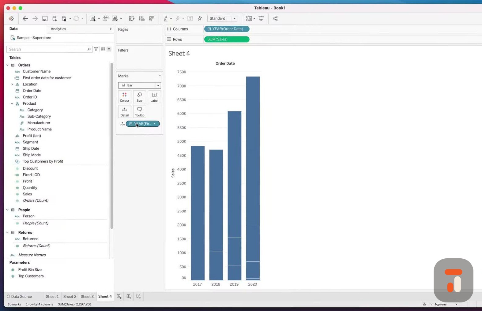
22:49where this comes handy is if we now build a
22:51slightly different visualization and note
22:54when
22:54i build this visualization i won't have
22:56customer anywhere in the visualization okay
22:59so let's just
23:00go in here and let's grab sales and i'm
23:02just going to put this onto rose and you'll
23:05see you just get
23:06one bar over time and what i'd like to do
23:09is show how many of my customers are repeat
23:13customers over
23:14the years essentially okay and so what i
23:16might have done is i might have dragged
23:18order id but
23:19actually the thing i want to use here is
23:21the order day so if i drag order day into
23:24the columns you'll
23:25see that i get a nice simple line chart i'd
23:28like that as a bar chart so that i can add
23:30some context
23:31to this and so what i'm going to do now
23:33with the color shelf is i'm going to drag
23:35that first order
23:36day because essentially what this will do
23:38is it will give me the year of the first
23:41order day for
23:42each and every customer okay so i can
23:44actually see let's say if the customer
23:46first ordered in 2017 it
23:48will mark that one color if they ordered in
23:502018 another color and so on and so forth
23:53but it will
23:53continue to do that for all their
23:55subsequent orders as you saw in the table
23:57but i don't have
23:58customer anywhere here in the visualization
24:01level of detail so let's drag that here
24:03onto color and
24:04now you can see that working in full force
24:06so you can see here that of course in my
24:08first year of
24:09business every customer was from that year
24:11so 100 okay and then in subsequent years
24:14that number has
24:15changed and so we can even do things like
24:17calculate the percentage of total for each
24:20year here i can
24:20just go back into some of sales do a quick
24:23table calculation do percentage of total
24:25and of course
24:26it will do this from left to right doing
24:28table across so these numbers here are the
24:30totals across
24:31the whole data set i actually want it
24:33differently i actually wanted to compute
24:34the percentage of
24:35total within each year and so what i can do
24:38is i can do a very quick cheat here and
24:41just do table
24:42down and that will do it vertically from
24:43the top to the bottom of this table which
24:45is just once
24:46each year essentially and then i can
24:48actually grab that number and put it on
24:51label and now i can
24:52confidently tell you that in 2018 77
24:55percent of our customers were first-time
24:58customers in 2017
25:00and so on and so forth and so you can start
25:02to see how you can use this for things like
25:05cohort
25:05analysis which is a very common type of
25:07analysis that you'd like to do and it hasn
25:09't taken me long
25:10to do any data prep whatsoever okay so the
25:13fundamental thing here is that lod's allow
25:16you
25:16to do calculations at a different level of
25:19detail to what's in the visualization the
25:22fixed level of
25:23detail is the only one of the level of
25:25detail calculation that works independent
25:27of what's in
25:28the view even if the dimension you're using
25:30is actually in the view if that makes sense
25:33okay now
25:34the last thing is that the fixed lod allows
25:36us to prescribe the level of detail and so
25:39it's really
25:40useful for telling tableau how to aggregate
25:42something or how to calculate something and
25:45then
25:45use that in context of another calculation
25:47you've seen me create two versions which is
25:49a very basic
25:50percentage of total and in this one we've
25:53done a very simple cohort analysis
25:55visualization just
25:56using the minimum order date for each
25:59customer doing that as an lod and then
26:01using that throughout
26:02our data set to give us some context for
26:05what's going on okay so hopefully that's
26:07been a useful
26:08guide for how to use the fixed level of
26:10detail and hopefully a decent introduction
26:12to level of detail
26:13calculations now these get very complex
26:15very quickly and so what i'm always going
26:18to do at
26:18the end of these videos is obviously show
26:20you some resources that you can go to to
26:22get a little bit
26:23more in-depth analysis and in-depth insight
26:25into how these functions work let's just go
26:28over here
26:28to tableau and if i just go here and i type
26:33in tableau level of detail there's a whole
26:37world of
26:38resources okay the first one is obviously
26:40the page itself and that tableau created
26:42for documentation
26:43it's really really good it has so much
26:45useful context in here and if you're the
26:48kind of person
26:48that loves detail and precision this is the
26:51page for you because tableau detail
26:53everything that
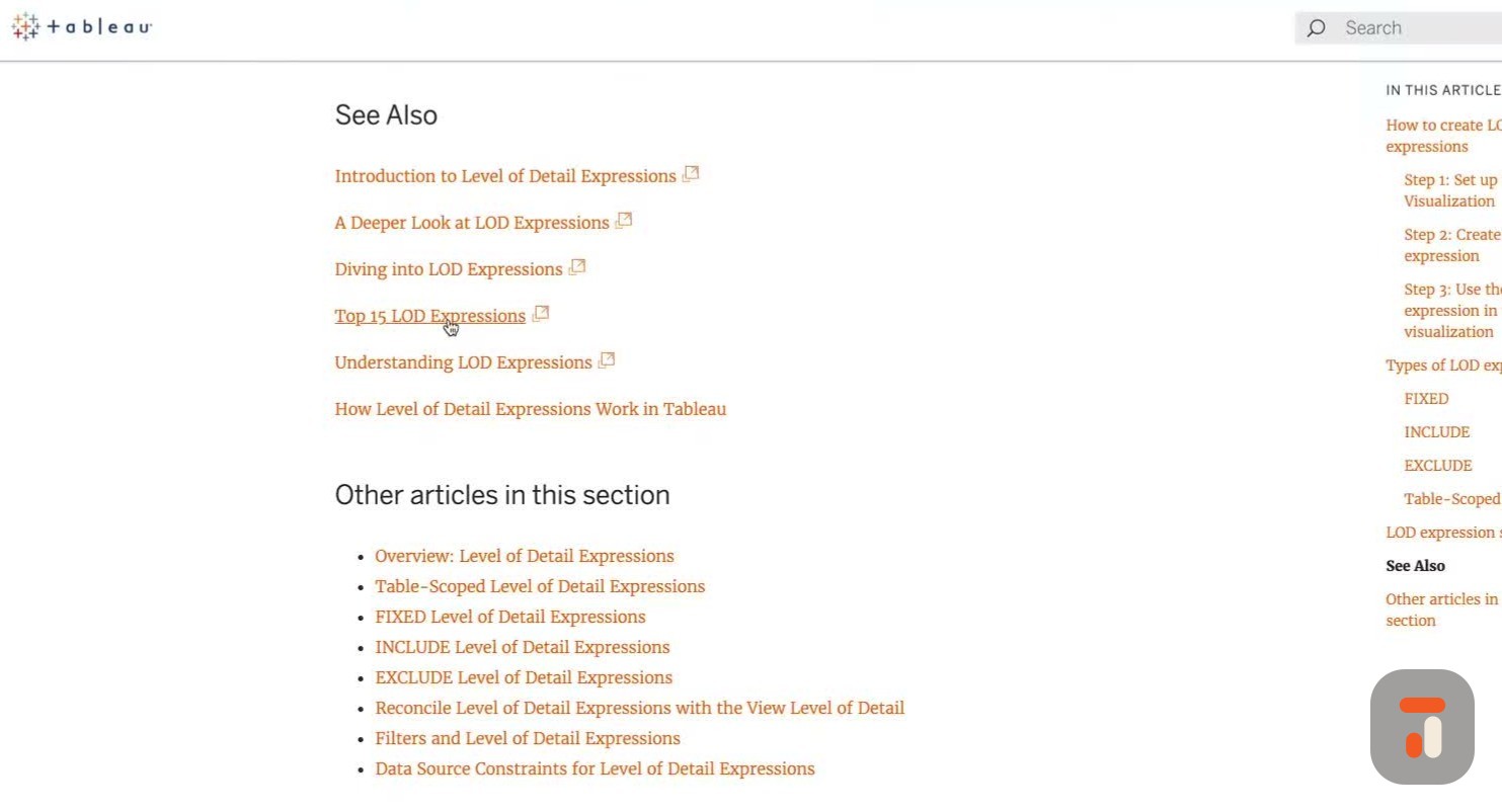
26:54is involved with level of details and if
26:57you go to the very end if i go to see also
26:59you'll see
27:00that tableau also link off to other white
27:02papers and other articles that you can go
27:04off and read
27:05more about the one i'd actually encourage
27:07everyone to have a look at is this top 15 l
27:10od expressions
27:11now i haven't covered exclude and include
27:13yet i'll do those very soon but essentially
27:16here you can
27:16see all the different types of questions
27:19that you might answer and ask as a business
27:21with lods okay
27:22and so this is really really good if we've
27:24just done this cohort analysis here for
27:26example that's
27:27a really sort of common one but you might
27:29also have other examples that you know are
27:31kind of
27:32questions that you've thought hey this is a
27:34really simple thing to do right and then
27:35you've actually
27:36tried it and it's not done exactly what you
27:38've expected that's probably because lods is
27:40what
27:40was missing from your sort of knowledge and
27:42information a percentage of total we just
27:44did
27:45this one as well and that's a very basic
27:47one new customer acquisitions very common
27:49one comparative
27:50analysis there's also this concept called
27:52proportional brushing where you can show
27:54something
27:55in context of a slightly bigger sort of
27:58part as well and so just check out each and
28:01every one of
28:01these concepts if all you did was read
28:03about these and just know about them then
28:05you'll know exactly
28:06where to come to in the future if you ever
28:08get stuck now another thing to bear in mind
28:10is that
28:10there are some restrictions if i go to this
28:13second link here go to how level of details
28:16expressions
28:17work in tableau they actually have a little
28:19bit more context as to how it's actually
28:21doing the
28:22calculation in the background and if you
28:24scroll down it gives you this sort of
28:26explanation i gave
28:27you before of you know the viz level of
28:29detail and what's going on and then also if
28:31i keep going down
28:32it also talks about limitations of level of
28:34detail so things that you have to watch out
28:37for and if
28:38you're working with these now the the thing
28:39about limitations is you know them when you
28:41hit them
28:42because you'll realize something's not
28:43happening so this is the kind of page to
28:44just be aware about
28:46if you try an lod and it's not working the
28:48way you've expected the other thing is to
28:50be aware of
28:51that lods don't work for every single data
28:53source if i just scroll all the way down
28:56you see that
28:56tableau actually lists which data sources
28:59and databases support lods and which ones
29:01don't
29:02now the typical database that you'd use to
29:04genuinely do so you know amazon redshift
29:07you know
29:07microsoft sql server and supported beyond
29:10certain versions and so essentially if you
29:12're using the
29:13latest database and you're using the most
29:15modern version of that database generally
29:17speaking it
29:18will be supported but for things like cubes
29:20um which tend to be slightly cumbersome to
29:22work with
29:23and actually lock in that kind of
29:24information anyway you'll find that there's
29:26actually a few
29:27restrictions there just to be aware of and
29:29just to sort of make sure you look at
29:31before you get
29:32stuck in so i'll put these three links in
29:34the description the first one is this level
29:36of detail
29:36page the second one this article about the
29:39top 15 lod expressions and the last one
29:41which gives you
29:42some context about some of the restrictions
29:45in level of detail calcs okay so hopefully
29:47that's
29:47been a useful introduction into the fixed
29:49level of detail in the next video we'll
29:51look at include and
29:52exclude and which are slightly easier but
29:55maybe slightly more of a sort of a mental
29:57mind maze to
29:58kind of get your head around okay if you've
30:00enjoyed this video you know what to do like
30:02subscribe share the video with someone who
30:04might find it useful and if you've got any
30:06comments
30:07please leave them below i'd love to get
30:08your comments i always love the feedback
30:10that i get
30:10positive or negative and it's really useful
30:12context for me and for other people who
30:14watch
30:15the videos and as always i'll catch you in
30:17the next video take it easy