 Tableau | Data visualisation
 How to build Scatter plot in Tableau | Tableau Charts
Build a fully formatted scatter plot in Tableau in just two minutes, complete with sets and trend lines.
- Place two continuous measures on rows and columns to create the basis of a scatter plot, then add a dimension like country to detail to split it into individual points
- Tableau aggregates measures by default as a sum, so switch to average when your data spans multiple years to get meaningful comparisons
- Convert continuous year to discrete and add it to detail to spread points out and convey the story better
- Format marks to a single circle, reduce size and opacity, and add a white border to handle overlapping data points
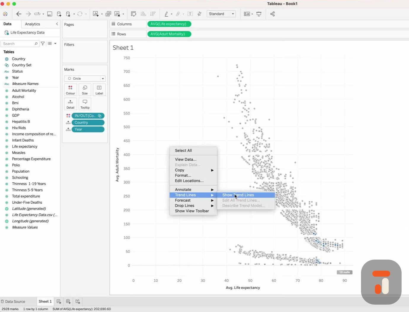
- Create a set of selected countries on colour and add trend lines to compare correlation between those countries and the rest of the world
Hey, it’s Tim here. Let me walk you through how to build a scatter plot in Tableau in roughly two minutes. I’m working with life expectancy data again, but this time we’re looking at some slightly different comparisons.
Start by taking adult mortality and putting it on columns, then take life expectancy and put it on rows. At this point you get a single data point, and technically that’s already a scatter plot. It isn’t telling us much yet, so we need to add context.
Drop country onto detail and you’ll get a dot for every country. Now a story starts to emerge. It’s important to notice that Tableau is aggregating these values using its default aggregation, a sum. You can change the default aggregation across the board, but here I’ll just change it in the chart to average. Because the data spans multiple years, averaging gives us a more sensible picture.
If you want the years on the chart too, you’ll notice they come through as continuous. Convert year to discrete, put it on detail, and now you get more dots that convey the story better.
Looking at the result, adult mortality climbs up the right-hand side and life expectancy climbs upwards too. That’s a slightly awkward way to read it, so I flip the chart round. With mortality going up the left and life expectancy running along the bottom, it makes more sense to me, because life expectancy on the x-axis reads like a scale from left to right.
Next, a bit of formatting. The marks are set to automatic and using multiple shapes, which we don’t need. Switch to a single circle, make it a little smaller, and because there’s quite a bit of overlap, bring the opacity down to around 78 percent. A white border makes all the dots easier to pick out.
This is where a scatter plot earns its keep. You can clearly see there’s no data falling around the 60, 70, 80 and 100 marks, along with some other gaps. Those disparities are too coincidental to be natural, which suggests something is happening in the data collection or storage that’s filtering certain points out.
To tell a richer story, you can add more context. Say I want to analyse a particular set of countries. I choose the United States and United Kingdom and compare them against every other country, which creates a set. Putting that set on colour highlights the dots representing those two countries.
Finally, add a trend line. Tableau looks at what’s on the colour pane and splits the trend line accordingly, so the blue is the United States and United Kingdom and the grey is every other country. Because we’re working with averages, this tells us more: the United States and United Kingdom have historically had fairly low adult mortality rates, so improving mortality has had less effect on life expectancy, whereas for most other countries there’s a much stronger correlation.
That’s pretty much it. Thanks for reading, and I’ll catch you in the next one.